Performing Linear Regression vs Time in TrendMiner

This Functional Tips & Tricks post was inspired by a Community question from Yves - the question can be found here.

Creating a Time Proxy Tag with Custom Calculations

In TrendMiner, scatter plots and regression tools require numeric X- and Y-axes. While most process tags (temperature, pressure, flow, etc.) are already numeric, time itself is not. This creates a challenge when you want to perform a linear regression of a tag versus time.

To solve this, we create a time proxy tag: a numeric tag that increases as time progresses over a defined window. Once this tag exists, it can be used on the X-axis of a scatter plot against any process tag on the Y-axis, enabling linear regression and trend analysis.

Why a Time Tag Is Required

TrendMiner’s scatter plots do not allow timestamps directly on the X-axis. Instead, both axes must be numeric tags. Therefore, to analyze temperature vs time, we must first convert time into a numeric variable.

This numeric time tag:

• increments as time advances

• is aligned with the process data

• and exists only within the time window of interest

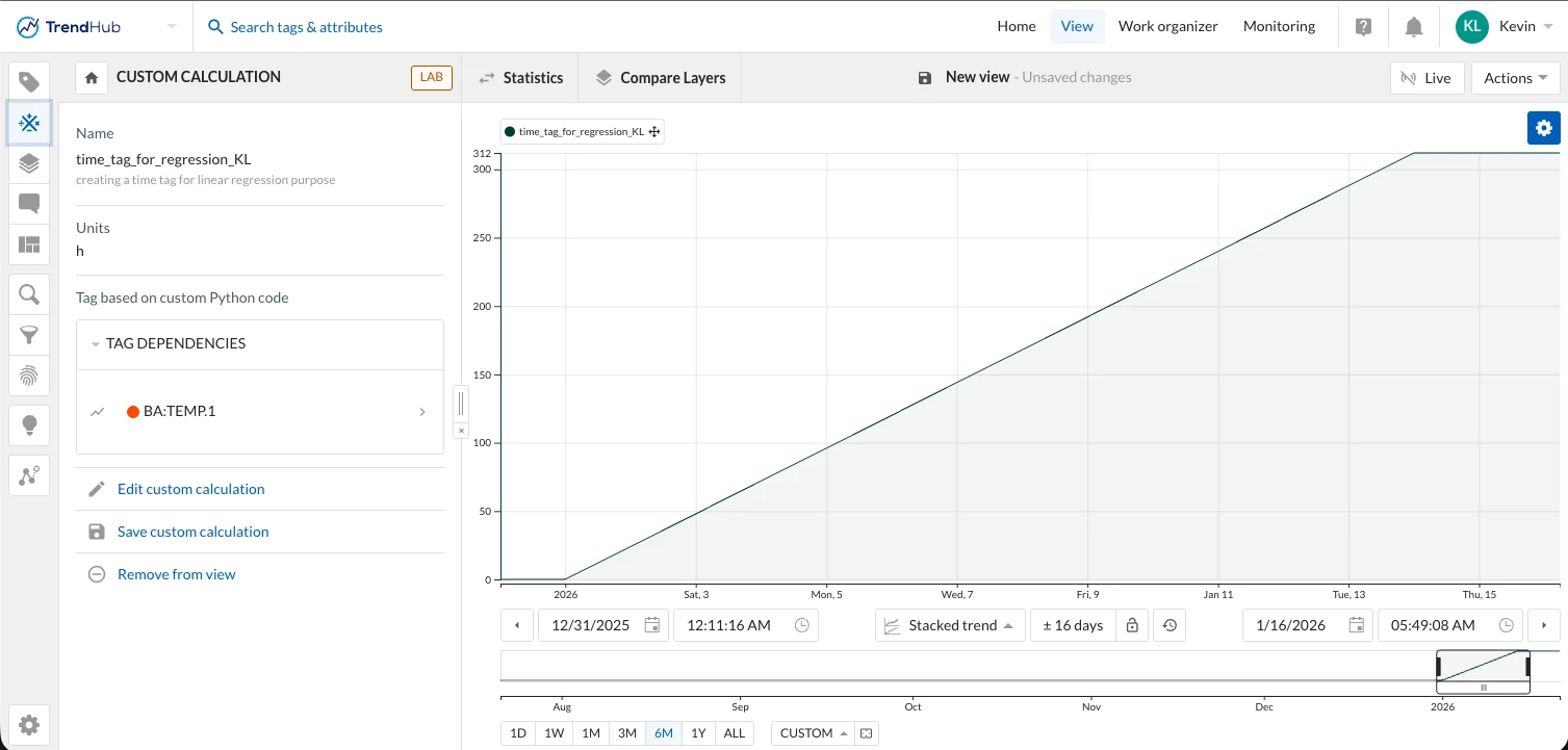
Using Custom Calculations (Expert License Feature)

To create this time proxy tag, we use Custom Calculations, a feature available with the TrendMiner Expert license.

Custom Calculations allow you to:

• write Python code in a sandboxed Jupyter environment

• retrieve existing tag data

• compute new values

• write the result back as a new tag

In this case, we use Python to compute hours since a fixed anchor start date and output that as a new tag.

Conceptual Approach

1. Use an existing tag (e.g., temperature) only to obtain timestamps

2. Define a fixed anchor start and end time

3. Compute hours since anchor start

4. Restrict the time counter to a defined window

5. Output the result as a new tag

This ensures:

• a monotonic time variable

• no resets due to internal execution chunking

• a clean numeric axis for regression

Code Walkthrough

Below is the full implementation used in the Custom Calculations sandbox with embedded comments.

import os
import pandas as pd
import numpy as np
from trendminer import TrendMinerClient

client = TrendMinerClient.from_token(
    token=os.environ["ACCESS_TOKEN"],
    tz="America/Chicago",
)

index_interval = client.time.interval(
    os.environ["START_TIMESTAMP"],
    os.environ["END_TIMESTAMP"],
)

# retrieve process tag for timestamps
temp_tag = client.tag.get_by_name("BA:TEMP.1")
temp = temp_tag.get_data(index_interval, resolution="1m").dropna()

# define regression start and end timestamp (fixed anchor dates)
anchor_start = pd.Timestamp("2026-01-01 00:00:00", tz="America/Chicago")
anchor_end   = pd.Timestamp("2026-01-14 00:00:00", tz="America/Chicago")

# compute hours since anchor start
x_hours = (temp.index - anchor_start).total_seconds() / 3600.0

# mask: only keep values inside the window, else 0
in_window = (temp.index >= anchor_start) & (temp.index <= anchor_end)

# preference: 0 value after the regression window, or hold last value after the regression window
# switch the comment structure if you want 0 value after anchor end
# x_hours = np.where(in_window, x_hours, 0.0)  # 0 before anchor start, increasing during window, 0 after anchor end
x_hours = np.clip(
    x_hours,
    0.0,
    (anchor_end - anchor_start).total_seconds() / 3600.0
)  # 0 before anchor start, increasing during window, holds final value after anchor end

# (optional) also prevent any tiny negative due to timezone/index quirks
x_hours = np.maximum(x_hours, 0.0)

# output the new tag
out = pd.Series(x_hours, index=temp.index, name="value")
out.index.name = "ts"
out.to_csv(os.environ["OUTPUT_FILE"])

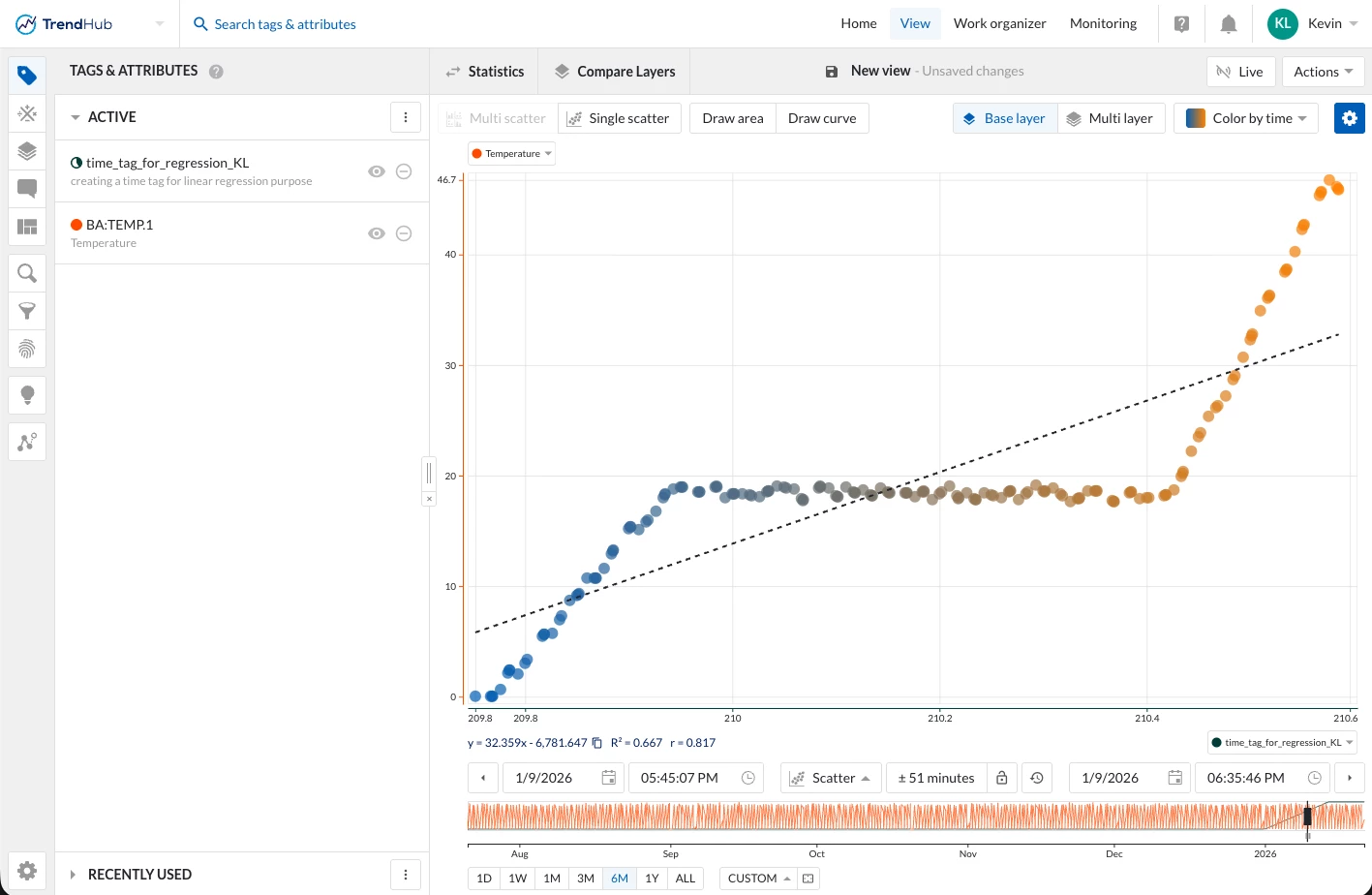
Using the Time Tag in TrendMiner

Once created:

• Use the time proxy tag on the X-axis

• Use temperature (or any process tag) on the Y-axis

• Enable TrendMiner’s linear trendline on the scatter plot

You now have a clean linear regression of a tag vs time.